How Do You Change Sample Size In Spss

One-Sample T-Test using SPSS Statistics

Introduction

The one-sample t-test is used to make up one's mind whether a sample comes from a population with a specific mean. This population mean is not e'er known, simply is sometimes hypothesized. For case, you want to show that a new teaching method for pupils struggling to learn English grammer tin can improve their grammar skills to the national average. Your sample would be pupils who received the new education method and your population mean would be the national boilerplate score. Alternately, yous believe that doctors that work in Accident and Emergency (A & E) departments work 100 hour per week despite the dangers (e.thousand., tiredness) of working such long hours. You sample 1000 doctors in A & E departments and run across if their hours differ from 100 hours.

This "quick start" guide shows you lot how to carry out a one-sample t-test using SPSS Statistics, every bit well equally interpret and report the results from this test. However, earlier we introduce you to this procedure, yous need to understand the different assumptions that your data must run into in order for a one-sample t-examination to requite you a valid upshot. We discuss these assumptions side by side.

SPSS Statistics

Assumptions

When you cull to analyse your data using a 1-sample t-exam, part of the process involves checking to make sure that the data you want to analyse can actually be analysed using a one-sample t-test. You lot demand to do this because it is but appropriate to use a one-sample t-exam if your information "passes" four assumptions that are required for a one-sample t-examination to give yous a valid effect. In practice, checking for these four assumptions just adds a little bit more fourth dimension to your analysis, requiring you to click a few more buttons in SPSS Statistics when performing your analysis, as well every bit remember a little bit more about your data, but it is not a hard task.

Before nosotros innovate you to these four assumptions, practise not be surprised if, when analysing your ain information using SPSS Statistics, one or more of these assumptions is violated (i.e., is not met). This is not uncommon when working with real-world data rather than textbook examples, which oftentimes only show you how to deport out a one-sample t-test when everything goes well! Still, don't worry. Even when your data fails sure assumptions, there is frequently a solution to overcome this. First, let'due south take a look at these four assumptions:

• Assumption #1: Your dependent variable should be measured at the interval or ratio level (i.e., continuous). Examples of variables that meet this criterion include revision time (measured in hours), intelligence (measured using IQ score), test performance (measured from 0 to 100), weight (measured in kg), and so along. Y'all can learn more than about interval and ratio variables in our article: Types of Variable.
• Assumption #2: The data are independent (i.east., not correlated/related), which ways that in that location is no human relationship betwixt the observations. This is more than of a study design outcome than something you tin can test for, but information technology is an of import assumption of the i-sample t-test.
• Assumption #3: There should exist no meaning outliers. Outliers are data points within your information that do non follow the usual pattern (e.thousand., in a study of 100 students' IQ scores, where the mean score was 108 with only a small variation between students, 1 educatee had a score of 156, which is very unusual, and may even put her in the top i% of IQ scores globally). The problem with outliers is that they tin have a negative effect on the one-sample t-exam, reducing the accuracy of your results. Fortunately, when using SPSS Statistics to run a one-sample t-test on your data, y'all can easily discover possible outliers. In our enhanced one-sample t-test guide, nosotros: (a) bear witness yous how to notice outliers using SPSS Statistics; and (b) discuss some of the options y'all have in order to deal with outliers.
• Assumption #4: Your dependent variable should be approximately normally distributed. Nosotros talk virtually the 1-sample t-test only requiring approximately normal data because it is quite "robust" to violations of normality, pregnant that the supposition tin can be a little violated and still provide valid results. Y'all tin can examination for normality using the Shapiro-Wilk test of normality, which is easily tested for using SPSS Statistics. In addition to showing yous how to exercise this in our enhanced one-sample t-examination guide, we likewise explicate what y'all tin do if your information fails this assumption (i.e., if it fails it more than a piffling bit).

You can bank check assumptions #3 and #iv using SPSS Statistics. Before doing this, yous should make sure that your data meets assumptions #one and #ii, although you don't demand SPSS Statistics to practise this. When moving on to assumptions #3 and #4, we suggest testing them in this society because information technology represents an order where, if a violation to the assumption is not correctable, y'all will no longer be able to use a one-sample t-test. Just call up that if yous practise not run the statistical tests on these assumptions correctly, the results you get when running a one-sample t-test might not be valid. This is why we dedicate a number of sections of our enhanced one-sample t-test guide to help you become this right. You lot can detect out about our enhanced content on our Features: Overview folio.

In the section, Process, we illustrate the SPSS Statistics procedure required to perform a i-sample t-test assuming that no assumptions have been violated. First, we set out the instance we utilize to explicate the one-sample t-exam procedure in SPSS Statistics.

SPSS Statistics

Example and Setup in SPSS Statistics

A researcher is planning a psychological intervention study, but earlier he gain he wants to characterise his participants' depression levels. He tests each participant on a item depression index, where anyone who achieves a score of 4.0 is deemed to take 'normal' levels of depression. Lower scores betoken less depression and higher scores bespeak greater depression. He has recruited 40 participants to take office in the study. Depression scores are recorded in the variable dep_score. He wants to know whether his sample is representative of the normal population (i.e., exercise they score statistically significantly differently from 4.0).

For a one-sample t-test, there will merely be one variable's information to be entered into SPSS Statistics: the dependent variable, dep_score, which is the depression score.

SPSS Statistics

Test Procedure in SPSS Statistics

The 5-stride Compare Means > One-Sample T Test... process below shows you how to analyse your data using a one-sample t-test in SPSS Statistics when the four assumptions in the previous department, Assumptions, have not been violated. At the terminate of these v steps, we show yous how to translate the results from this test. If you lot are looking for help to brand sure your data meets assumptions #iii and #4, which are required when using a ane-sample t-test, and can be tested using SPSS Statistics, you can larn more in our enhanced guides on our Features: Overview page.

Since some of the options in the Compare Means > One-Sample T Test... procedure changed in SPSS Statistics version 27, we show how to carry out a one-sample t-test depending on whether you lot have SPSS Statistics versions 27 or 28 (or the subscription version of SPSS Statistics) or version 26 or an earlier version of SPSS Statistics. The latest versions of SPSS Statistics are version 28 and the subscription version. If you are unsure which version of SPSS Statistics yous are using, meet our guide: Identifying your version of SPSS Statistics.

SPSS Statistics versions 27 and 28
and the subscription version of SPSS Statistics

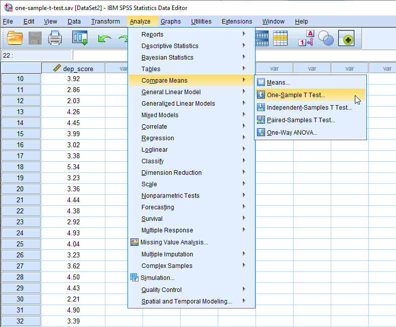
1. Click Analyze > Compare Means > One-Sample T Test... on the principal carte:

   

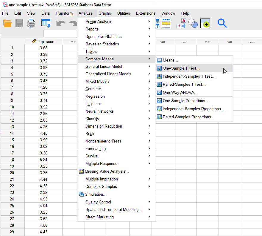
   Published with written permission from SPSS Statistics, IBM Corporation.

   
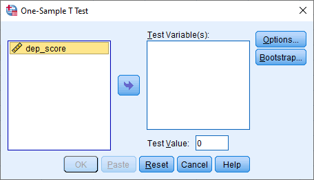
   You will be presented with the Ane-Sample T Exam dialogue box, as shown below:
   

   

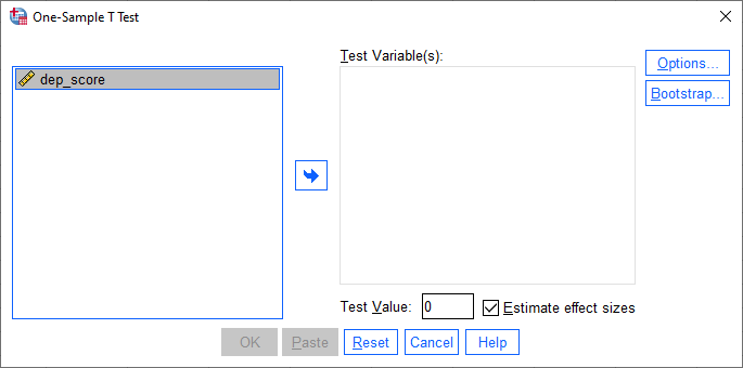
   Published with written permission from SPSS Statistics, IBM Corporation.

2. Transfer the dependent variable, dep_score, into the Test Variable(s): box by selecting it (past clicking on it) and and then clicking on the button. Enter the population mean you are comparing the sample against in the Test Value: box, by changing the electric current value of "0" to "4". Keep Due eaststimate effect sizes selected. You will end up with the following screen: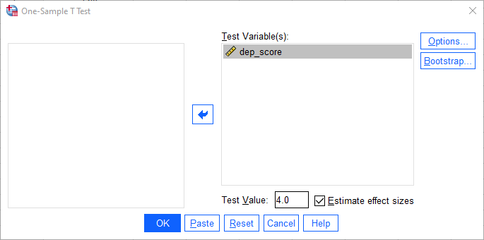

   

   Published with written permission from SPSS Statistics, IBM Corporation.

3. Click on the push button. You will be presented with the Ane-Sample T Test: Options dialogue box, every bit shown below: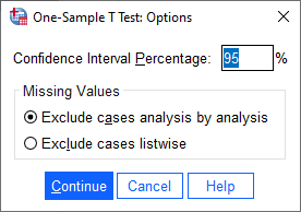

   

   Published with written permission from SPSS Statistics, IBM Corporation.

   
   For this example, keep the default 95% confidence intervals and Exclude cases analysis by analysis in the –Missing Values– area.

   Note 1: Past default, SPSS Statistics uses 95% conviction intervals (labelled as the Confidence Interval Percentage in SPSS Statistics). This equates to declaring statistical significance at the p < .05 level. If you wish to change this yous can enter any value from 1 to 99. For example, entering "99" into this box would result in a 99% conviction interval and equate to declaring statistical significance at the p < .01 level. For this instance, keep the default 95% confidence intervals.

   Note 2: If y'all are testing more than one dependent variable and you have any missing values in your information, you need to think carefully virtually whether to select Exclude cases analysis past assay or Exc50ude cases listwise) in the –Missing Values– area. Selecting the wrong option could mean that SPSS Statistics removes data from your analysis that you wanted to include. We discuss this further and what options to select in our enhanced i-sample t-examination guide.

4. Click on the button. You lot will be returned to the 1-Sample T Test dialogue box.
5. Click on the push to generate the output.

Now that you accept run the Compare Means > One-Sample T Exam... procedure to bear out a one-sample t-examination, go to the Interpreting Results department. You lot can ignore the section below, which shows you how to carry out a one-sample t-test if you lot have SPSS Statistics version 26 or an earlier version of SPSS Statistics.

SPSS Statistics version 26
and before versions of SPSS Statistics

1. Click Analyze > Coyardpare Means > 1-Saplenty T Test... on the main menu:

   

   Published with written permission from SPSS Statistics, IBM Corporation.

   
   You will exist presented with the Ane-Sample T Test dialogue box, as shown below:
   

   

   Published with written permission from SPSS Statistics, IBM Corporation.

2. Transfer the dependent variable, dep_score, into the Test Variable(s): box by selecting it (by clicking on it) and then clicking on the button. Enter the population mean you are comparing the sample against in the Test Value: box, by changing the electric current value of "0" to "4". You will end up with the post-obit screen: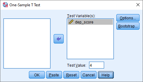

   

   Published with written permission from SPSS Statistics, IBM Corporation.

3. Click on the button. You volition exist presented with the Ane-Sample T Test: Options dialogue box, as shown beneath: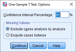

   

   Published with written permission from SPSS Statistics, IBM Corporation.

   
   For this case, keep the default 95% conviction intervals and Exclude cases analysis by analysis in the –Missing Values– area.

   Note i: By default, SPSS Statistics uses 95% confidence intervals (labelled equally the Confidence Interval Percentage in SPSS Statistics). This equates to declaring statistical significance at the p < .05 level. If you lot wish to change this you can enter whatever value from i to 99. For example, entering "99" into this box would result in a 99% confidence interval and equate to declaring statistical significance at the p < .01 level. For this example, keep the default 95% confidence intervals.

   Note 2: If yous are testing more than 1 dependent variable and you have any missing values in your data, you lot demand to recollect carefully nigh whether to select Exclude cases analysis by analysis or Exclude cases listwise) in the –Missing Values– area. Selecting the incorrect choice could mean that SPSS Statistics removes data from your analysis that you wanted to include. Nosotros discuss this further and what options to select in our enhanced one-sample t-test guide.

4. Click on the push button. You volition be returned to the One-Sample T Examination dialogue box.
5. Click on the button to generate the output.

SPSS Statistics

Interpreting the SPSS Statistics output of the i-sample t-exam

SPSS Statistics generates ii master tables of output for the ane-sample t-test that contains all the data you require to interpret the results of a 1-sample t-examination.

If your data passed assumption #3 (i.e., in that location were no pregnant outliers) and assumption #four (i.eastward., your dependent variable was approximately normally distributed for each category of the independent variable), which nosotros explained earlier in the Assumptions department, y'all will only need to interpret these two master tables. All the same, since you should take tested your information for these assumptions, you volition also need to translate the SPSS Statistics output that was produced when you lot tested for them (i.eastward., y'all will have to translate: (a) the boxplots you used to bank check if there were any significant outliers; and (b) the output SPSS Statistics produces for your Shapiro-Wilk test of normality to determine normality). If you practice not know how to do this, we show you in our enhanced one-sample t-test guide. Recollect that if your data failed any of these assumptions, the output that you get from the ane-sample t-test procedure (i.due east., the tables we discuss below), will no longer exist relevant, and you volition demand to translate these tables differently.

Nonetheless, in this "quick get-go" guide, we take y'all through each of the two primary tables in plow, assuming that your data met all the relevant assumptions:

Descriptive statistics

You can brand an initial estimation of the data using the One-Sample Statistics table, which presents relevant descriptive statistics:

Published with written permission from SPSS Statistics, IBM Corporation.

It is more than mutual than non to present your descriptive statistics using the mean and standard deviation ("Std. Deviation" column) rather than the standard error of the mean ("Std. Error Mean" column), although both are acceptable. Yous could written report the results, using the standard departure, as follows:

• General
• APA

Mean low score (3.72 ± 0.74) was lower than the population 'normal' depression score of 4.0.

Mean depression score (Chiliad = 3.72, SD = 0.74) was lower than the population 'normal' depression score of 4.0.

However, by running a 1-sample t-test, you are really interested in knowing whether the sample you lot have (dep_score) comes from a 'normal' population (which has a hateful of 4.0). This is discussed in the next section.

One-sample t-test

The One-Sample Test table reports the result of the one-sample t-test. The top row provides the value of the known or hypothesized population mean you lot are comparing your sample data to, as highlighted beneath:

Published with written permission from SPSS Statistics, IBM Corporation.

In this case, you tin run across the 'normal' depression score value of "4" that you entered in earlier. You now demand to consult the first iii columns of the 1-Sample Examination tabular array, which provides information on whether the sample is from a population with a hateful of 4 (i.e., are the means statistically significantly unlike), as highlighted below:

Published with written permission from SPSS Statistics, IBM Corporation.

Moving from left-to-right, y'all are presented with the observed t-value ("t" column), the degrees of freedom ("df"), and the statistical significance (p-value) ("Sig. (2-tailed)") of the 1-sample t-test. In this instance, p < .05 (information technology is p = .022). Therefore, it can be concluded that the population means are statistically significantly dissimilar. If p > .05, the divergence between the sample-estimated population mean and the comparing population mean would not be statistically significantly dissimilar.

Note: If you see SPSS Statistics country that the "Sig. (two-tailed)" value is ".000", this actually ways that p < .0005. It does not hateful that the significance level is actually zero.

SPSS Statistics likewise reports that t = -ii.381 ("t" column) and that there are 39 degrees of freedom ("df" cavalcade). You need to know these values in order to report your results, which you could do equally follows:

• General
• APA

Depression score was statistically significantly lower than the population normal low score, t(39) = -2.381, p = .022.

Low score was statistically significantly lower than the population normal depression score, t(39) = -ii.381, p = .022.

The breakdown of the terminal role (i.east., t(39) = -2.381, p = .022) is every bit follows:

	Part	Meaning
1	t	Indicates that we are comparing to a t-distribution (t-test).
2	(39)	Indicates the degrees of liberty, which is N - 1
three	-two.381	Indicates the obtained value of the t-statistic (obtained t-value)
iv	p = .022	Indicates the probability of obtaining the observed t-value if the null hypothesis is correct.
Tabular array four.ane: Breakdown of a one-sample t-test statistical statement.

Yous tin can also include measures of the deviation between the two population means in your study. This information is included in the columns on the far-correct of the I-Sample Test table, as highlighted below:

Published with written permission from SPSS Statistics, IBM Corporation.

This section of the table shows that the mean deviation in the population ways is -0.28 ("Mean Difference" column) and the 95% confidence intervals (95% CI) of the difference are -0.51 to -0.04 ("Lower" to "Upper" columns). For the measures used, it will be sufficient to report the values to ii decimal places. Yous could write these results equally:

• General
• APA

Low score was statistically significantly lower by 0.28 (95% CI, 0.04 to 0.51) than a normal depression score of 4.0, t(39) = -ii.381, p = .022.

Low score was statistically significantly lower past a mean of 0.28, 95% CI [0.04 to 0.51], than a normal depression score of 4.0, t(39) = -2.381, p = .022.

Standardised effect sizes

Later on reporting the unstandardised effect size, we might also report a standardised outcome size such every bit Cohen's d (Cohen, 1988) or Hedges' g (Hedges, 1981). In our case, this may exist useful for future studies where researchers want to compare the "size" of the effect in their studies to the size of the event in this study.

In that location are many different types of standardised upshot size, with different types often trying to "capture" the importance of your results in dissimilar ways. In SPSS Statistics versions 18 to 26, SPSS Statistics did not automatically produce a standardised event size as part of a one-sample t-test assay. Withal, it is easy to calculate a standardised effect size such as Cohen's d (Cohen, 1988) using the results from the one-sample t-test analysis. In SPSS Statistics versions 27 and 28 (and the subscription version of SPSS Statistics), two standardised effect sizes are automatically produced: Cohen's d and Hedges' k , as shown in the One-Sample Effect Sizes tabular array below:

Published with written permission from SPSS Statistics, IBM Corporation.

SPSS Statistics

Reporting the SPSS Statistics output of the one-sample t-test

You can report the findings, without the tests of assumptions, as follows:

• General
• APA

Mean low score (iii.73 ± 0.74) was lower than the normal depression score of four.0, a statistically significant difference of 0.28 (95% CI, 0.04 to 0.51), t(39) = -2.381, p = .022.

Mean low score (Chiliad = 3.73, SD = 0.74) was lower than the normal depression score of 4.0, a statistically significant mean difference of 0.28, 95% CI [0.04 to 0.51], t(39) = -2.381, p = .022.

Calculation in the information about the statistical test you ran, including the assumptions, you have:

• Full general
• APA

A one-sample t-test was run to make up one's mind whether depression score in recruited subjects was different to normal, defined equally a low score of 4.0. Depression scores were normally distributed, as assessed past Shapiro-Wilk's test (p > .05) and there were no outliers in the data, as assessed by inspection of a boxplot. Mean depression score (3.73 ± 0.74) was lower than the normal depression score of 4.0, a statistically meaning difference of 0.28 (95% CI, 0.04 to 0.51), t(39) = -2.381, p = .022.

A one-sample t-test was run to determine whether depression score in recruited subjects was different to normal, defined as a depression score of 4.0. Depression scores were usually distributed, every bit assessed by Shapiro-Wilk's examination (p > .05) and there were no outliers in the data, every bit assessed past inspection of a boxplot. Hateful depression score (M = 3.73, SD = 0.74) was lower than the normal depression score of 4.0, a statistically significant mean difference of 0.28, 95% CI [0.04 to 0.51], t(39) = -two.381, p = .022.

Aught hypothesis significance testing

You can write the outcome in respect of your null and culling hypothesis as:

• Full general
• APA

There was a statistically significant deviation between means (p < .05). Therefore, we can refuse the naught hypothesis and accept the alternative hypothesis.

There was a statistically significant difference between ways (p < .05). Therefore, we can reject the cipher hypothesis and accept the alternative hypothesis.

Practical vs. statistical significance

Although a statistically pregnant difference was establish between the low scores in the recruited subjects vs. the normal depression score, information technology does not necessarily hateful that the difference encountered, 0.28 (95% CI, 0.04 to 0.51), is enough to be practically significant. Indeed, the researcher might accept that although the departure is statistically significant (and would report this), the difference is non large plenty to be practically significant (i.e., the subjects can be treated as normal).

In our enhanced one-sample t-test guide, we show you lot how to write up the results from your assumptions tests and one-sample t-examination procedure if y'all demand to report this in a dissertation/thesis, assignment or research report. We do this using the Harvard and APA styles. We as well explain how to interpret the results from the One-Sample Effect Sizes table, which include the two standardised event sizes: Cohen's d and Hedges' g . You can learn more than well-nigh our enhanced content in our Features: Overview department.

How Do You Change Sample Size In Spss,

Source: https://statistics.laerd.com/spss-tutorials/one-sample-t-test-using-spss-statistics.php

Posted by: flowersdowanceares.blogspot.com

Share this post